
Quantum Composer as a research-assisting tool
Here, we present some of the scenarios where Composer has been or could be used as a research-assisting tool in the ultracold atoms field. That is, we present our (subjective) experiences with incorporating the tool's qualitative and quantitative capabilities into the different stages of a research project. In a certain sense, these have appreciable overlaps and parallels to repurposing citizen science games [1-2], which are inherently geared towards non-experts, into software useful for expert scientists [3]. The primary notion, in this case, is that software artifacts (distinctly different from e.g. the produced data) and design principles may emerge in developing for the former audience that can prove valuable also for the latter. Among others, the core tenets (e.g. flexibility, ease of use, rapid iterability) of Quantum Composer reinforce said ideas and remain central also in this context as elaborated in the following examples.
Theoretical research
A substantial amount of our research is geared towards quantum optimal control, [4-10] a mature, but evolving, field of research as it is one of the requisites for quantum technology experiments [11]. A common task in quantum optimal control is to steer an initial quantum state to a target state with desired accuracy in the most optimal way [4]. This is achieved by influencing the system dynamics through certain controls (e.g. the depth or center of an optical tweezer) that parameterize the Hamiltonian in a way specific to a given problem. Usually, optimal controls are found by iterative, local optimization of many different (often order 100-10000) initial guesses, or seeds. This paradigm, known as multistarted local optimization, typically involves large-scale parallel optimization processes on e.g. a computer cluster.
Quantum Composer includes the capability to set up, solve, and analyze such state transfer problems. Although not by itself suitable for advanced control techniques like multistarting, we have had very positive experiences with using the program both as a precursor for the simulation (problem definition), optimization, and analysis of the resulting optimal dynamics. As a concrete example, the control problem studied in Ref. [5] has a non-trivial dependence on some of the control parameters. We used Composer to e.g.
(1) probe different regimes and combinations of these parameters to deepen our understanding of the problem, which is useful in part for designing seeding strategies,
(2) confirm that the geometry was correctly modelled by comparing the energy spectrum to a benchmark paper,
(3) find proper boundaries for the control values for keeping lattice unit cells unmixed (a central assumption), and
(4) confirm unit conversions between simulation and SI units.
We used Composer for similar tasks in Ref. [6], which treats several single-particle and BEC control problems. There, we also estimated the timescale necessary for appreciable dynamics and used those results directly for related rough quantitative estimates included in the published paper. Additionally, we have performed numerous smaller, internal numerical studies in a wide variety of different contexts, e.g. for studying how the transmission and reflection of Gaussian wavepackets impinging on different types of potential barriers changes with the initial spatial and momentum distributions.
In principle, the above investigations and visualizations could be conventionally conducted by writing corresponding C++ native source code (assuming prior installation of library dependencies), writing compilation scripts, building and linking the program, running the executable, exporting the results, importing the results in an appropriate tool, writing visualization code, and finally executing it. This multi-staged procedure, however, ranges from being quite tedious to unrealistic, depending on the individual user's programming experience and needs. Especially, even for the most basic applications, only a fraction of the time is spent on dealing with the actual physical concepts and phenomena under consideration. Further, both programming and research are inherently fine-grained iterative processes,
each iteration changing often just a tiny bit of behavior, but nonetheless requiring invocation of the full pipeline. One of the defining core tenets of Composer, as highlighted throughout this paper, circumvents this chain by lowering the barrier for entry, containing the work space to a single application, allowing for rapid feedback on changes without re-building, and focusing on the visualization of physical concepts.
Overall, we find that, rather than being a complete replacement for text-based programming, Quantum Composer is a welcomed and effective addition in the suite of available tools at our disposal.
Experimental Research
We have found that Composer is also a useful tool for exploring experimentally-relevant potentials and the dynamics of quantum states within these potentials, especially if one is just beginning to work in research. For example, many dipole potentials used for atom trapping are generated with Gaussian laser beams [12]. How these potentials and their energy eigenstates are affected e.g. by the beam waist or laser power is straightforward to model in Composer. It is also trivial to add the effects of gravitational sag when determining whether or not a trap can hold up against gravity. One can also explore and optimize atom dynamics in such traps. This is a necessary precursor to actual experimental implementation, as one can simulate a system and verify its utility before undertaking the often expensive and time-consuming process of laboratory setup and testing. Thus, easy-to-use tools like Composer allow the experimentalist to perform such tests without the overhead of most numerical programming methods.
In our experimental research group, we found Composer to be a practical and useful tool for determining whether or not single atoms trapped in an optical lattice potential could be prohibited from tunneling to certain lattice sites using an attractive dipole potential. This problem is typically solved in practice by using a repulsive potential to remove a well and replace it with a potential barrier. Intuitively, it seems strange to plug a well to inhibit tunneling using attractive potentials. However, if one thinks of tunneling as the temporal evolution of a non-stationary state (e.g. a particle localized to a single well of a multi-well system), then it stands to reason that tunneling is inhibited if one shifts the energy states of a given well (or wells) out of resonance with the rest of the wells. The question remains, however, whether such potential shifting can be done without bringing higher-excited levels into resonance with the ground state of the un-shifted wells.
To illustrate this in Composer, we set up an eight-well system as shown in Fig. 1(a). This cosinusoidal lattice represents part of our (effectively) infinite optical lattice potential in which we trap single atoms. The lattice potential is given by 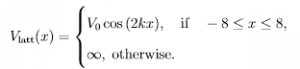
Here, we include the hard wall boundaries to avoid any confusion due to edge effects, as Composer uses a combination of absorbing and periodic boundary conditions (cf. the Reference pages). We define our spatial coordinate such that x lies between -10 and 10. It is good practice to work with potentials that tend towards infinity at the boundaries to preserve numerical accuracy and physicality of simulations.
For the purposes of this simulation, the lattice depth is $V_0 = 5E_\mathrm{rec}$, where the recoil energy is defined as $E_\mathrm{rec} = \hbar^2k^2/2m$ for a lattice with wavenumber $k = 2\pi/\lambda$, wavelength $\lambda = 1064$ nm, and the mass here refers to $m_\mathrm{Rb} = 1.44\times 10^{-25}$ kg, the mass of the rubidium-87 atoms we trap in our experiment [13]. Note that $E_\mathrm{rec} = 1$ in this simulation. The lattice depth is low enough that we do not expect tunneling to be fully suppressed due to the superfluid-to-Mott-insulating transition in one dimension (the other two dimensions are fully frozen out) [14]. As we expect to populate only one atom per site when preparing our states, however, these simulations are single-particle and neglect any nonlinearity due to the fact that we load Bose-condensed atoms into the lattice. However, similar investigations of BEC dynamics are possible in Composer.
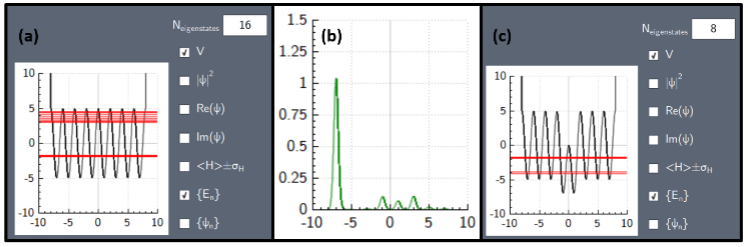
Figure 1. (a) Energy plot showing the 8-well lattice potential (black) and the energy landscape for the first 16 eigenstates (red lines), (b) Position Plot showing the state (green) localized as much as possible to the first well, (c) Another Energy Plot showing the lattice potential with the Gaussian plug, showing that the lowest band has been split, and two energies now sit below the original lowest band shown in (a).
The energy landscape of this potential is shown in Fig. 1(a), and we see that the first 16 eigenstates make up two bands of energies trapped in the lattice. By creating an equal superposition of all states trapped in the first band (8 total eigenstates), we can create an approximation to a state localized in the first well of the lattice, as shown in Fig. 1(b). The ``leakage'' of this state into other wells is a consequence of the finite number of wells considered in this simulation.
To illustrate the effect of well plugging, we superpose on this potential a Gaussian potential (representing a laser-created dipole potential) of the form
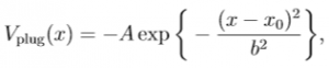
i.e. the total potential is $V(x) = V_\mathrm{latt} + V_\mathrm{plug}$, where we set the amplitude of the plug to $A = 5$ and its width to be $b = 1$ (noting that in scaled units, each lattice site spans half of a wavelength, corresponding to 2 spatial units in the simulation). If we center the plug potential around zero, that is, $x_0 = 0$, we expect that wells 4 and 5 (counting wells 1,...,8 starting from the left) will be plugged. Indeed, the energy spectrum of the superposed state, shown in Fig. 1(c) shows 6 states remaining in the original lowest band, but two states have been shifted lower in energy and thus out of resonance with this band. By clicking on the ${\psi_n}$ checkbox, the user can verify that the two different bands correspond to states localized in the plugged and unplugged wells, respectively.
The time-evolution of the state in Fig. 1(b) without (with) the plug are shown in Fig. 2 (Fig. 3). Because the initial state is not completely localized to a single well, we plot the integrated population in three sections of the lattice: to the left of the plug (wells 1-3), in the plug (wells 4-5), and to the right of the plug (wells 6-8). As expected, the majority of the initial state lies in wells 1-3.
Without the plug, the wave function evolves such that it is non-negligibly present in all wells at some time, and thus the population evolves between the three sections of the lattice. This makes sense intuitively, as the localized wave function is a superposition of all 8 states in the lowest band, and each of the 8 eigenstates is delocalized in the lattice. With the plug, however, the state population stays within the respective sections. Thus, the plug not only prevents population on either side from moving through to the other side, but movement into or out of the plug section is also restricted, even though it is classically attractive.
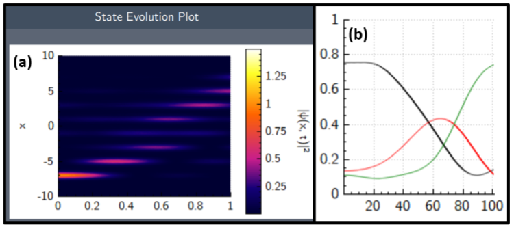
Figure 2. (a) State Evolution Plot showing the probability density (y-axis) of the lattice wave function in the unplugged (A = 0) potential as time evolves (x-axis). (b) Scalar Time Trace Plot showing the total integrated population to the left of the plug (wells 1-3, black), inside the plug (wells 4-5, red), and on the other side of the plug (wells 6-8, green). Without the plug, the wave function tunnels freely throughout the entire lattice.
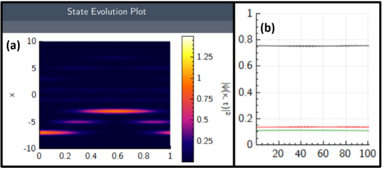
Figure 3. Same as Fig. 2, but for the plugged potential (A =5). The wave function is now prohibited from tunneling into and out of the (attractive) plug.
This simulation is certainly a simplified case of the actual experiment, but it allows us as experimental researchers to quickly simulate complex scenarios that move beyond simple back-of-the-envelope calculations without the use of complex numerical software. Indeed, we have experienced that what is shown here could feasibly be implemented and understood by an advanced Bachelor's student doing a project in our lab. For reference, the flowscene used in this section can be downloaded and explored here.
References
[1] S. Cooper et al, "Predicting protein structures with a multiplayer online game,'' Nature, 466 (7307), 756--760 (2010).
[2] Jinseop S. Kim et al, "Space–time wiring specificity supports direction selectivity in the retina.'' Nature 509, 331–-336 (2014).
[3] Seth Cooper et al, "Repurposing Citizen Science Games as Software Tools for Professional Scientists,'' Association for Computing Machinery, Proceedings of the 13th International Conference on the Foundations of Digital Games, 39, 1--6 (2018).
[4] J. J. Sørensen et al, "QEngine: A C++ library for quantum optimal control of ultracold atoms,'' Comp. Phys. Comm. 243, 135--150 (2019).
[5] Jesper H. M. Jensen et al, "Time-optimal control of collisional $\sqrt{SWAP}$ gates in ultracold atomic systems,'' Phys. Rev. A 100, 052314-1--13 (2019).
[6] Jesper H. M. Jensen et al, "Crowdsourcing human common sense for quantum control,'' arXiv:2004.03296, 1--24 (2020).
[7] J. H. M. Jensen et al, "Exact Gradients and Hessians for Quantum Optimal Control and Applications in Many-Body Matrix Product States,'' arXiv:2005.09943, 1--23 (2020).
[8] M. Dalgaard et al, "Global optimization of quantum dynamics with AlphaZero deep exploration,'' npj Quantum Information 6 (6), 1--9 (2020).
[9] J. J. Sørensen et al, "Quantum optimal control in a chopped basis: Applications in control of Bose-Einstein condensates,'' Phys. Rev. A 98, 022119 (2020).
[10] J. J. Sørensen et al, "Optimization of pulses with low bandwidth for improved excitation of multiple-quantum coherences in NMR of quadrupolar nuclei,'' J. Chem. Phys. 152, 054104-1--9 (2020).
[11] J. P. Dowling and G. J. Milburn, "Quantum technology: the second quantum revolution,'' Phil. Trans. R. Soc. Lond. A 361, 1655–-1674 (2003).
[12] R. Grimm, M. Weidemüller, and Y. B. Ovchinnikov, "Optical dipole traps for neutral atoms'' Adv. At. Mol. Opt. Phys. 42, 95--170 (2000).
[13] O. Elíasson et al, "Spatial tomography of individual atoms in a quantum gas microscope'' arXiv:1912.03079, 1--6 (2019).
[14] R. E. Sapiro, R. Zhang, and G. Raithel, "Reversible loss of superfluidity of a Bose–Einstein condensate in a 1D optical lattice'' New J. Phys. 11 013013-1--10 (2009).