Frequently Asked Questions

Why isn’t anything happening when I try to time-evolve my system?

There are two things that you can check here. First, your Time Evolution node should be in a For Loop scope, and the start and end points of your loop should correspond to the start and end points of your desired time evolution. Furthermore, $\Delta i$ corresponds to your time resolution, and this should not be set too high, otherwise you get unphysical results.

If your Time Evolution node is already in a For Loop scope and you have set your parameters correctly, try pressing the green Start button at the top left corner of the toolbar. This should start your system evolving in time.

Why is my time evolution seemingly choppy in updating?

The For Loop boundary node has a Pause Duration field that indicates the time in between finishing one iteration and moving on to the next. By default it is zero, in which case there is no guarantee for Plots etc. to update regularly. If this is an issue, try setting it to a small value like 0.0001.

Why can't I interact with the nodes?

In scenes that contain For Loops, you cannot interact with nodes after pressing the Play button because that could potentially lead to undefined behavior. A pop-up will show in the bottom region of the screen if you attempt to do this. To edit the scene further, click the red, circular arrow Reset button (or cmd+r or ctrl+r on the keyboard for macOS and Windows/Linux) next to the Play button. Note: this potentially erases the displayed results immediately.

Why does my For Loop or Grape Optimization output not compute?

For Loop and Grape Optimization output is only computed at the end of the loop, and is not recalculated at each iteration. If the outputs are used for subsequent computations, these calculations are performed when the output is available. For example, if a Grape Optimization outputs an optimized control which is then propagated over in a subsequent For Loop, the For Loop will run only once the initial optimization has stopped.

What happens at the spatial boundaries of a simulation?

When finding eigenenergies and eigenstates in the Spectrum node, non-periodic hardwall boundaries are used (the end points are not connected). This essentially means that the ends act as infinite square well potential. This exactly diagonalizes the Hamiltonian $H=T+V$ where $T$ uses the 5-diagonal approximation to the second derivative with error $\mathcal O(\Delta x^5)$.

Time evolution is implemented with so-called split-step Fourier transforms, which inherently applies periodic boundaries (the end points are connected). This essentially means that there is no infinite square well potential at the ends, and the wave function can travel through the edges i.e. move through one side and reappear at the other.

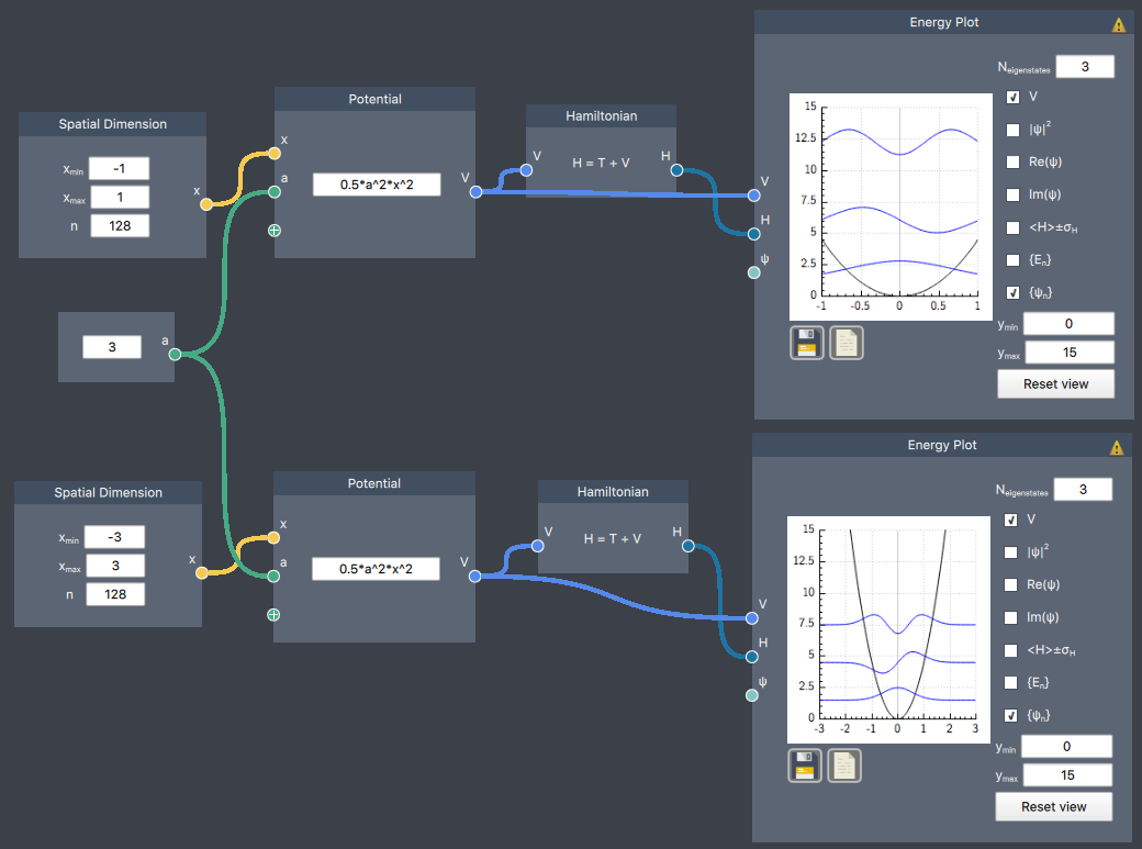
Because of these differences in boundary conditions (infinite potential at the ends or not), a state that is expected to be stationary may not be. The reason for the former choice is that the QEngine (the underlying simulation library) is used for studying trapping geometries in which the potential smoothly tends towards infinity at the edges. Compare the two cases in the screenshot below: the potential is the same, but if the spatial extent is not large enough (±1), the potential does not tend toward infinity quickly enough. Consequently, the eigenstates look like those of the infinite square well. When the spatial extent is large enough (±3), the potential tends toward infinity and the eigenstates look as expected (see also The energies and states I am getting are wrong! below).

As a rule of thumb, if the eigenstates do not sufficiently flatten out before reaching the edge, the implicit infinite well from the non-periodic boundaries are interefering with the intended potential expression.

Thus, the user must on a case-by-case scenario make sure that seemingly erroneous behavior is not related to the boundary conditions.

The energies and states I am getting are wrong!

If you are getting wrong answers, check the following (see also What happens at the spatial boundaries of a simulation?):

1. Is your potential running out of the space defined by the Spatial Dimension node? If so, increase the spatial limits of your flowscene.
2. Make sure that your spatial resolution is high enough. We suggest starting at 128 steps, but for potentials with large spatial limits or a lot of fine structures, higher resolution may be necessary to get accurate results.

The more rapidly the potential changes, the more resolution is generally required for numeric accuracy. Smooth potentials (e.g. harmonic) are much more easily simulated than 'jagged' potentials (e.g. infinite well).

Everything is so slow! What is happening?

As your flowscenes get more and more complicated, they may run more and more slowly. This is a natural part of doing numerical quantum mechanics. As with any other numerical software, some flowscenes will have a delicate balance between accuracy and resolution (both in space and time), especially if the potential you are working with requires fine resolution or you are working with nonlinear GPE dynamics.

In these cases, we would recommend experimenting with the space and time resolution. If you are getting accurate results at a lower resolution, there is no good reason why you should increase this resolution.

Sometimes, however, you’re stuck with a simulation that requires high resolution in space and/or time, and it may run slowly on your machine. In these cases, please just be patient! Composer will do what you are asking, but it takes time for the program to catch up with what you want. Try performing actions slowly and methodically, and wait for one action (e.g. changing a parameter or deleting a node) to complete before moving on to the next action.

When I evolve in time, the wave function becomes spiky and jittery! What is happening and how do I stop it?

This is a symptom of numerical inaccuracies (see also The energies and states I am getting are wrong!). In particular, smooth potentials (e.g. harmonic) allow larger time steps that still faithfully represents the correct dynamics, whereas non-smooth potentials (e.g. infinite well) requires relatively small time steps to obtain physically correct results.

If you experience spikiness or jitters, you can try choosing a lower time step. However, this may not the best approach because the simulation will then take a long time to run. Often the preferred fix to this problem is to use smoothed versions of the non-smooth potentials, see www.quatomic.com/composer/reference/quantum-composer-basics/expressions/. This allows much higher time steps while remaining conceptually faithful to the original potential.

When I open my .flow file, I don’t see anything, but I know I made something in the file! Where is my work?

Sometimes Composer likes to hide things off screen. Use the mouse wheel to zoom out, and you’ll probably find your flowscene happily waiting for you. You can then center your cursor over the flowscene and zoom back in again.

I want to save a plot inside a loop, but I can't click the save button without resetting the simulation (and thus clearing the plot). What do I do?

Place the plot outside the scope containing the loop. It will not update until after the node is finished running, but it will also not clear its data after resetting. You can then save the data in the plot. Unfortunately, plots that update each time the loop runs (like Scalar Time Trace plots of optimization fidelities) cannot be saved. This will be fixed in an upcoming version.