Scalar Time Trace Plot

Description

The Scalar Time Trace Plot node plots a scalar quantity developing over time.

Input

The node has the following inputs:

• Time (t): The scalar quantity that outputs the time update
• Scalar quantity (a): Any scalar quantity developing over time. More than one scalar quantity can be added as denoted by the + in the inputs. 

Content 

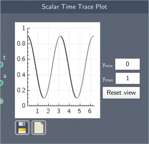
The primary content is the plot of the scalar quantity developing over time. The plot can be saved and its data can be exported as a .$csv$ file.

Additionally, the node has two content-fields that define the limits of the $y$-axis of the plot. The 'Reset view' button re-sets the $y$-axis limits to its default values. 

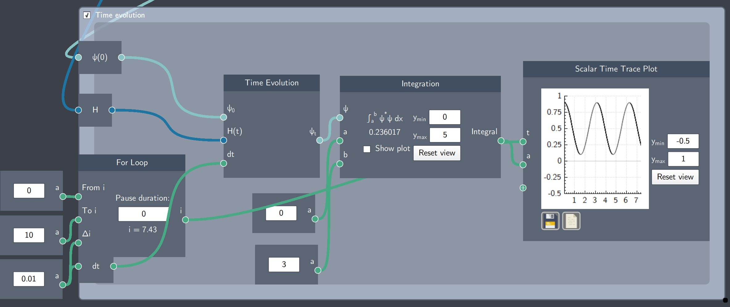
Example 

In the example below, the integral of the probability density of a time-evolving state is plotted in the Scalar Time Trace Plot. The input 't' is taken from the output (i) of the For Loop node and the value of the integral (Integration node)at every time step (t) is applied as a scalar input (a).