Control
Description
The Control node contains configurable control curves, which enters the potential $V=V(x,u_1,u_2,\dots)$. Controls are either used as seeds in Grape Optimization or dynamically evolved over in For Each Control Value.
Input
The node has the following input:
- Time (t): This input defines the scalar values for the time axis
Content
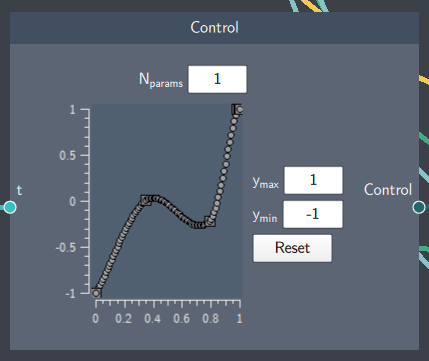
The number of controls is defined by $N_{params}$. Each control parameter can be independently manipulated: left-clicking on the curve adds a control anchor which can be dragged vertically, right-clicking an anchor removes it. The control range is specified in the $y_{min}$ and $y_{max}$ fields. The Reset button takes removes all intermediate anchors and sets the control curve to be flat and centered in the control range.
Output
- Control: This node outputs all the control values within the range of the discretized control curve
Example
In the example below, a harmonic potential is parameterized by two controls $V(u_1,u_2) = \frac{1}{2}u_1^2 (x-u_2(t) - 0.25 \cos(10\pi t))^2$, where $u_1$ controls the harmonic frequency and $u_2$ the trap center, which is also modulated by an additional (uncontrolled) cosine term. The Control node defines the time dependent shapes $u_1(t/t_{\mathrm{max}})$ and $u_2(t/t_{\mathrm{max}})$, which are roughly parabolic and linear, respectively. In the For Each Control Value scope, the control curves are iterated in time and the instantaneous values are output in the For Each Control Value boundary node. These are plotted in the Scalar Time Trace Plot and are used as inputs to the Potential which can be used for Time Evolution.