State Evolution Plot

Description

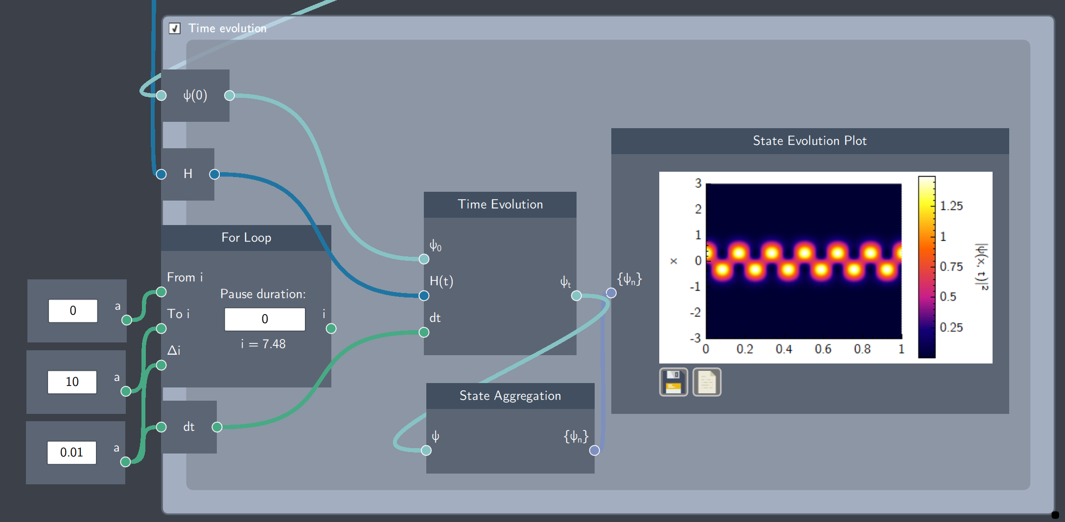
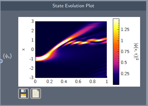
The State Evolution Plot is used to visualize the evolution of the probability density of a state over space and time.

Input

The node has the following input:

• Time-evolving state ($\psi_n$): A state evolving dynamically over time

Content

The plot displays the probability density evolving over space (y-axis) and time (x-axis) as a color density plot. The colorbar denotes the range of the probability density, which can be used to read the plot. The horizontal axis denotes time and the vertical axis denotes space  (defined by the spatial dimension in the simulation). The plot can be saved and its data can be exported as a .$csv$ file by clicking on the icons on the plot.

Example 

In the example below, the State Evolution Plot plots the probability density as a function of time for an initial state $\psi = \psi_0 + \psi_1$ in a harmonic oscillator. The visualization shows how the density periodically oscillates back and forth.