For Each Control Value
Description
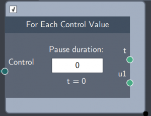
The For Each Control Value scope takes a control curve and iterates over each the control values. It can be used to show the time dynamics of any Control, e.g. a seed or an optimized control from Grape Optimization
Input
The node has the following input:
- Control: Control curve(s) defined in the Control node.
Content
This node is a time loop which displays the time based on the time dimensions and timestep defined in the Time node. For every value of $t$, the node outputs the instaneous control values contained in the input Control.
Output
The number of control value outputs equals $N_\mathrm{params}$ in the input Control.
- Time (t): The scalar values of the time axis
- Control value (u1): The control value corresponding to time $t$
- Control value (u2): The control value corresponding to time $t$
- ...
Example
In the example below, a harmonic potential is parameterized by two controls $V(u_1,u_2) = \frac{1}{2}u_1^2 (x-u_2(t) - 0.25 \cos(10\pi t))^2$, where $u_1$ controls the harmonic frequency and $u_2$ the trap center, which is also modulated by an additional (uncontrolled) cosine term. The Control node defines the time dependent shapes $u_1(t/t_{\mathrm{max}})$ and $u_2(t/t_{\mathrm{max}})$, which are roughly parabolic and linear, respectively. In the For Each Control Value scope, the control curves are iterated in time and the instantaneous values are output in the For Each Control Value boundary node. These are plotted in the Scalar Time Trace Plot and are used as inputs to the Potential which can be used for Time Evolution.