GRAPE optimization
Description
The GRAPE Optimization scope refers to a gradient-based optimization algorithm known as Gradient Ascent Pulse Engineering (GRAPE), and is relevant for quantum optimal control problems. It is an optimization loop which optimizes the control path based on the inputs provided. The simulation is started by clicking the green Run button.
Inputs
The node has the following inputs:
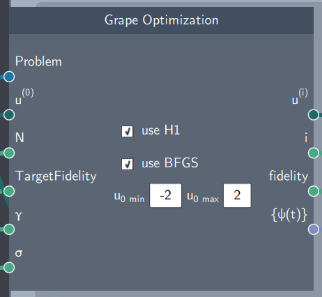
- Problem: A control problem defined by an initial state, a target state, and a potential expression
- Initial control ($u^{(0)}$): An initial control curve defined in the Control Node
- Number of Iterations (N): The number of iterations to be run by the optimization algorithm
- Target Fidelity: The optimization algorithm will run until the target fidelity is achieved
- Regularization parameter ($\gamma$): A real scalar value that penalizes rapid temporal fluctuations in the control field
- Weight factor ($\sigma$): A real scalar value that penalizes controls outside the bounds
Content
The node has two checkboxes: H1 and BFGS, which enable the choice of search direction. The search direction is based on the gradient information, which are the gradients calulated in iterations 1,2....N. It also has fields to specify the bounds of each control.
Output
- Iterated control ($u^{(i)}$): The updated control at the $i^{th}$ iteration
- Iteration number (i): A real scalar value corresponding to the iteration number
- Fidelity: The fidelity achieved at the $i^{th}$ iteration
- State evolved over the current control ({$\psi(t)$}): The aggregate of states over time $t$
Example (control_ex_opt.flow)
In the example below, the frequency ($u_0$) and trap center ($u_1$) of a harmonic oscillator potential is controlled to transfer a ground state at $u_1=-3$ to translated ground state at $u_1 = 3$. The states are supplied to the Control Problem node, which itself defines the potential expression. The problem is input along initial control curves (a seed defined in a Control node) and optimization parameters to the Grape Optimization. The initial cruve (blue) and the optimized path (red) are plotted together in the Control Comparison Plot. As the simulation runs, the fidelity is plotted against the iteration number in Scalar Time Trace Plot, the optimized control is re-plotted, and the probability density is shown for all $t$ in State Evolution Plot.
The initial fidelity is very low ($F=0.017$), but after optimizing it reaches $F=0.99$. After reaching this fidelity, the optimization stops and outputs the optimized control which is then used input to a For Each Control Value scope, plotting the time evolution in real time.