State Comparison Plot

Description

The State Comparison Plot node plots any two states for comparison.

Input

The node has the following inputs:

Potential ($V$): The Potential node where the potential function is defined
State 1 ($\psi$): Any analytically defined or linearly-combined wave function
State 2 ($\varphi$): Any analytically defined or linearly-combined wave function

Content

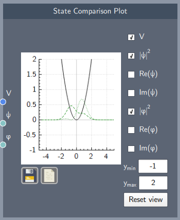
This plot consists of check-boxes corresponding to different functions, which can be selected to visualize them.

The different check-boxes/functions from top to bottom (with required inputs in parenthesis) are:

Show/Hide the potential (V)
Show/Hide the probability distribution of state 1($\psi$)
Show/Hide the real part of state 1($\psi$)
Show/Hide the imaginary part of state 1 ($\psi$)
Show/Hide the probability distribution of state 2 ($\varphi$)
Show/Hide the real part of state 2 ($\varphi$)
Show/Hide the imaginary part of state 2 ($\varphi$)

Additionally, the $y$-axis limits can be set to any limits and reset to the original limits as well. The plot can be saved and the data can be exported as a $.csv$ file.

Output

The output of the node is the visualisation in the plot based on the inputs and selection of the check-boxes.

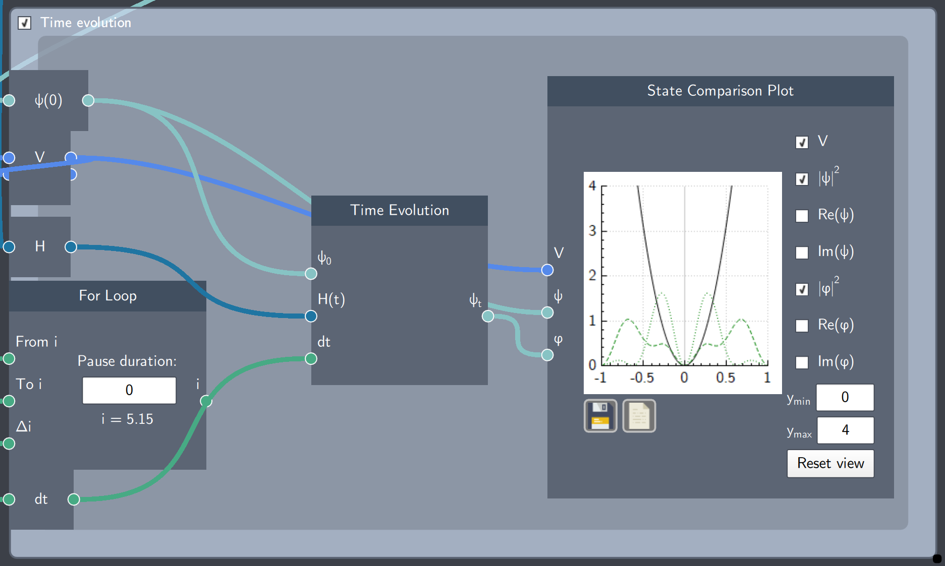
Example

In the example below, the probability densities of two states are plotted inside a time evolution scope. The first state $\psi$ (green dotted-curve) is the initial state of the system (a non-stationary state of the harmonic oscillator) and the second state $\varphi$ (green dashed-curve) is the time-evolved state.