Expressions
Several nodes in the Composer allow for writing mathematical functional expressions. This page outlines the allowed expressions.
Note: spaces are ignored in expressions, so they can be placed wherever.
There are two types of function expressions: scalar functions and functions of $x$ (defined in Spatial Dimension)
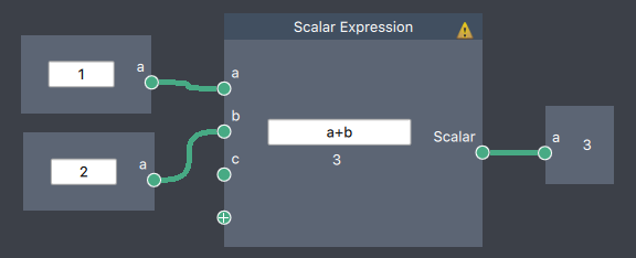
- Scalar function: takes an optional number of scalar inputs and outputs a scalar
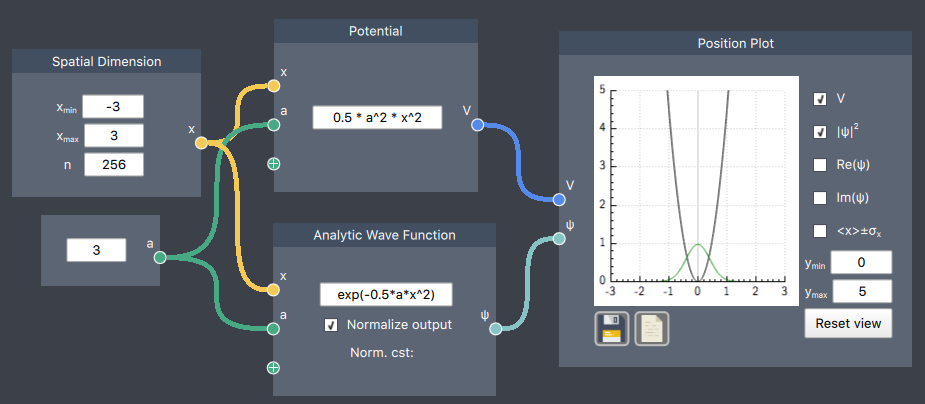
- Function of $x$: takes $x$ as a required input and an optional number of scalar inputs and outputs a vector with the expression evaluated at the corresponding $x$ values
Scalar function
Functions of $x$
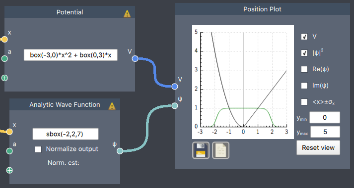
The most common usage of expressions is in defining Potentials $V(x)$. Defining Analytical Wave Functions is somewhat less common, since one often to express $\psi(x)$ as Linear Combinations of Hamiltonian eigenstates (i.e. the Spectrum). Most of the following is thus mainly meant to address the creation of potentials, but can be equally applied to the creation of states.
Helpful expressions for potentials
We provide special functions for several potentials.
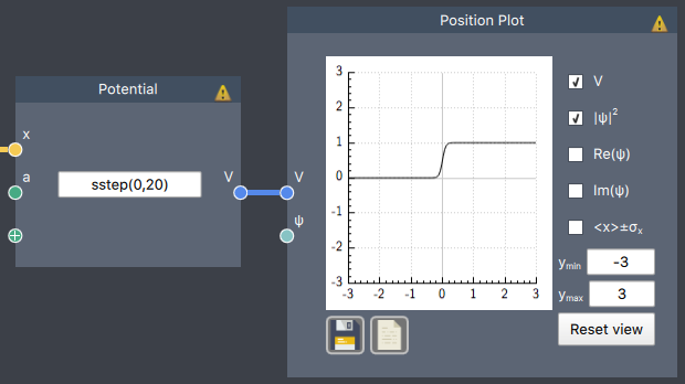
Numerical simulations of non-smooth functions, such as the box and the step function, are prone to numerical instabilities, especially when performing time evolution. This can be alleviated by using smoothed versions of the functions. We provide two such functions, prefixed with 's' for smooth.
infinite(a,b) = $\begin{cases} 0, \quad a < x < b \\ \infty, \quad \text{otherwise} \end{cases}$

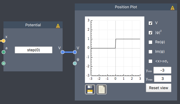
step(a) = $\begin{cases} 0, \quad x < a \\ 1, \quad \text{otherwise} \end{cases}$
sstep(a,h) = $\frac{1}{1+exp(-h\cdot(x-a))}$
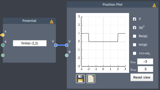
finite(a,b) = $\begin{cases} 0, \quad a < x < b \\ 1, \quad \text{otherwise} \end{cases}$
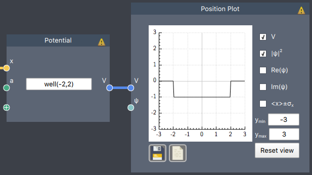
well(a,b) = $\begin{cases} -1, \quad a < x < b \\ 0, \quad \text{otherwise} \end{cases}$
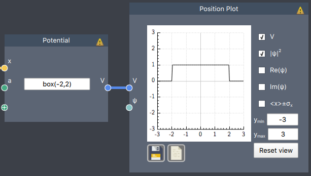
box(a,b) = $\begin{cases} 1, \quad a < x < b \\ 0, \quad \text{otherwise} \end{cases}$
sbox(a,b,h) = sstep(a,h)-sstep(b,h)

Constants
pi = 3.14159265358979323846
i = 0+1i
e = exp(1)
Arithmetic operator precedence
operators with lower precedence are calculated before those with higher precedence
1: ^
2: unary +, unary -
3: *, /
4: +, -
Basic functions
Basic functions are implemented both for scalars and $x$ and can be used in any expression. The variable $a$ can mean either in the following list:
- pow(a,b) = $a^b$
- sqrt(a) = $\sqrt{a}$
- abs(a) = $|a|$
- exp(a) = $e^a$
- exp2(a) = $2^a$
- log(a) = $\log (a)$
- log2(a) = $\log_2(a)$
- log10(a) = $\log_{10}(a)$
- sin(a)
- cos(a)
- tan(a)
- asin(a) = $\sin^{-1}(a)$
- acos(a) = $\cos^{-1}(a)$
- atan(a) = $\tan^{-1}(a)$
- sinh(a)
- cosh(a)
- tanh(a)
- asinh(a) = $\sinh^{-1}(a)$
- acosh(a) = $\cosh^{-1}(a)$
- atanh(a) = $\tanh^{-1}(a)$
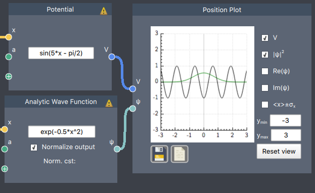
Gaussian wave function in a sine potential
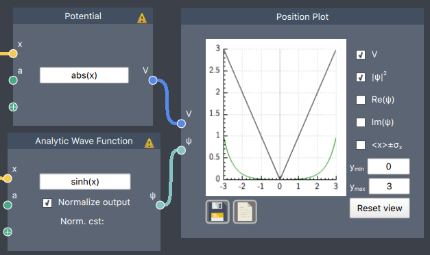
sinh wave function in an absolute value potential
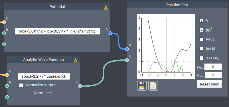
Combining Expressions
Valid expressions can be added, subtracted, multiplied, divided, or passed as arguments to enclosing functions. This allows a large flexibility of defining and studying systems numerically which would otherwise be either very hard or impossible to do analytically. For illustration, here is an example of combining more and more expressions to obtain complex functions: